The Journey #4: Monitoring and prescribing resistance training using movement velocity: Part 1

In one of the first articles in this series, we mentioned potential issues with a traditional approach to resistance training monitoring and prescription. We focused on two issues that are related to the inability of the traditional approach to account for daily readiness to train. In another article, we covered how movement velocity (i.e., the velocity of the concentric muscle action during exercise) can reflect how your athletes or clients feel about the loads they are supposed to lift on a given day. Additionally, your athletes or clients will probably slow down when they start approaching muscle failure during exercise, so movement velocity can also reflect how many repetitions they can do in a set on a given day. Both scenarios can fall under the daily readiness to train umbrella term. Therefore, it seems that movement velocity can solve the issues with the daily fluctuations in readiness we mentioned previously. Indeed, to circumvent the identified issues with the traditional approach to resistance training monitoring and prescription, sport scientists have recommended the velocity-based approach to resistance training (a.k.a velocity-based training or VBT) [1]. As it is hopefully clear by now, this approach prides itself in considering the daily readiness of your athletes and clients [1]. Without further ado, let’s finally dive into how to use movement velocity to monitor and prescribe RT and account for daily fluctuations in readiness.

Understanding the load-velocity relationship

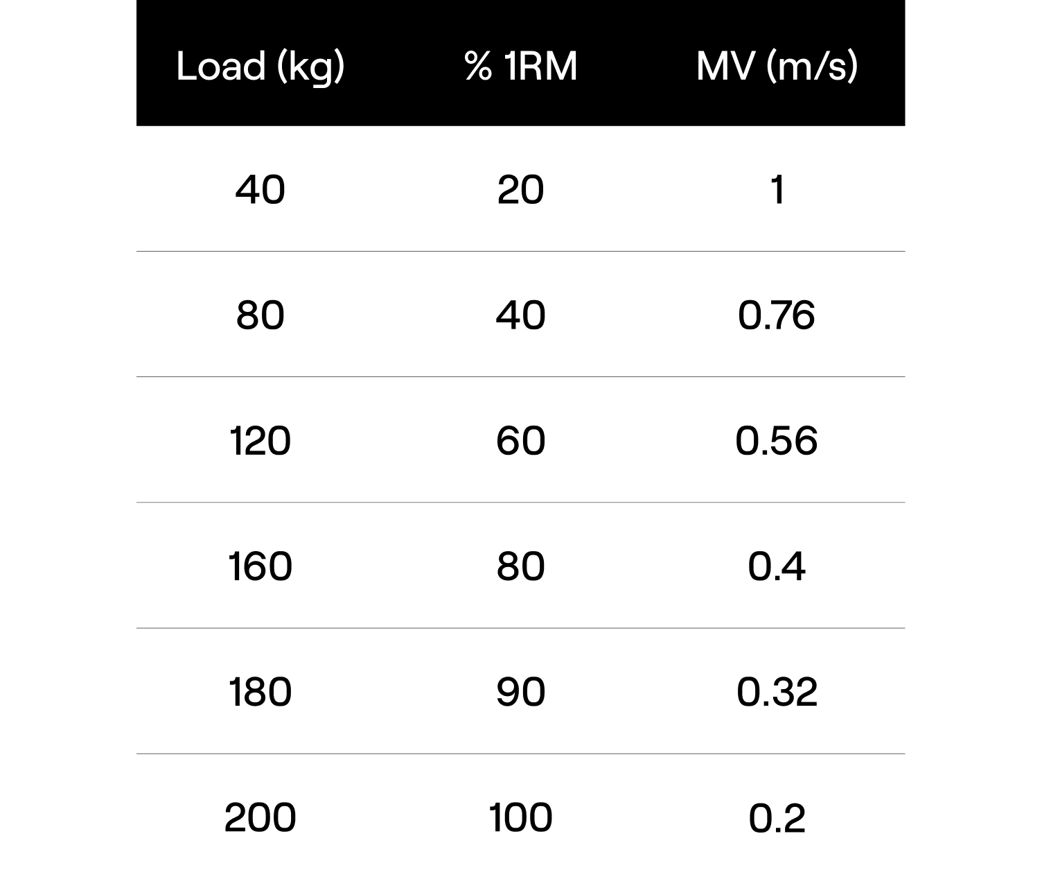
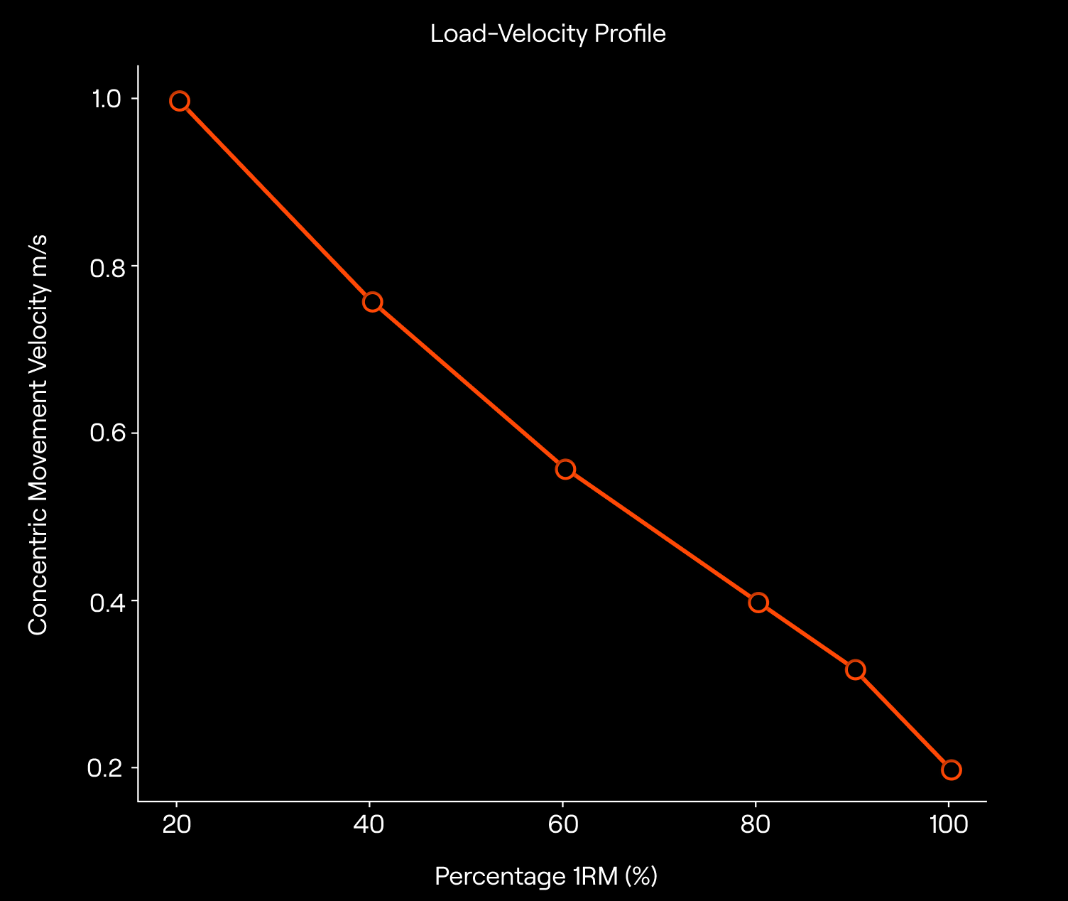
Let’s start with the loads. How can we use movement velocity to prescribe loads during resistance training? The entire premise of VBT relies upon the inverse (almost perfectly) linear relationship between the load and movement velocity. In other words, heavier loads cannot be lifted with the same velocity as lighter loads [1, 2, 3]. Remember, with movement velocity, we refer to the velocity of the concentric muscle action during the exercise. This inverse relationship makes sense; we can all agree that our athletes or clients will lift 70% of their one-repetition maximum (1RM) faster than 90% of their 1RM. But how can we use this information to monitor and program resistance training? The first step would be to conduct an incremental loading test (i.e., the 1RM test) with your athletes or clients in the exercise of choice. Wait a minute, how is this different from the traditional approach for which we highlighted several issues already? Well, the important thing is to record the movement velocity of the repetitions during the 1RM test to create a so-called load-velocity profile (LVP). There are many ways to conduct a 1RM test and thus establish the LVP of your athletes or clients. A very common procedure reported in the literature consists of performing three repetitions with 20, 40, and 60% of a self-estimated 1RM (i.e., estimated by your athletes or clients), one repetition with 80 and 90% of a self-estimated 1RM, followed by no more than five 1RM attempts [2, 3]. Once you have conducted the test with your athlete or a client, you can store the data on their absolute loads, self-estimated percentages of 1RM, 1RM, and associated movement velocities you recorded in a spreadsheet (e.g., Microsoft Excel). Since you now know the 1RM of your athlete or a client, you can convert the submaximal loads into the actual percentages of their 1RM and substitute them with the self-estimated ones in the table. Then, since you have three data points for 20, 40, and 60% of 1RM (because you have three repetitions with each load), the common practice is to pick the fastest repetition and discard others (more on that later). You could then plot the relationship between absolute/relative loads and corresponding velocities by drawing the line of the best fit (i.e., the linear regression). To get an idea of how the table with data and the corresponding plots would look like, please see below:

Before we move on with the utility of the LVP we just created, we need to highlight two things. In the previous article, we discussed the importance of lifting with maximal intended velocity or with maximal intent during the concentric phase of the exercise. This is especially important when establishing the LVP. Why? Well, imagine if your athlete or client did not lift their self-estimated 20, 40, and 60% of 1RM with the maximal intent. Chances are that the movement velocity with all three loads could have been very similar, despite the obvious differences in loads. Using such data to create an LVP would be misleading and ultimately wrong. Secondly, when creating an LVP for an athlete or client, we mentioned that we’re only keeping the fastest repetition out of the three with 20, 40, and 60% of 1RM. We do that because it can sometimes be hard for our athletes and clients to lift the light loads as fast as possible and be consistent at the same time with their movement velocity. Therefore, it’s an established practice to keep only the fastest repetition (and its corresponding velocity) from each set with submaximal loads. Okay , with those two caveats cleared out of the way, let’s continue with the utility of the LVPs.

What is the minimal velocity threshold and how can we use it to predict 1RM?

Let’s have a look at the table we previously created. Looking at the bottom of it, we see the 1RM of our athlete or a client and the movement velocity associated with it. This movement velocity is often referred to as minimal velocity threshold (MVT) which can be used in the equation of our regression (i.e., LVP) line to predict the 1RM of our athletes and clients on a daily basis. There are many approaches to 1RM predictions using the LVP and MVT of an athlete or client. The two most popular are the so-called “multiple-point” and the “two-point” methods. The former requires our athlete or a client to perform several warm-up sets with increasing submaximal loads (e.g., 20-40-60-80-90%, 40-60-80-90%, or 20-40-60-80% 1RM) whereas the latter requires our athletes or clients to perform only two warm-up sets with distant loads (e.g., 45 and 85% of 1RM in order to have a light and heavy load). Which method should you use will depend upon your context. The multiple-point method is probably a safer choice for those of you who don’t want to risk it because having more data points is (almost) always better. If you’re time-constrained, then the two-point method is an obvious choice at the potential expense of slightly lower accuracy. Now, regardless of the 1RM prediction method used, it is important to note that the findings on their accuracy are equivocal. Namely, some research groups concluded that the multiple- or two-point methods are valid whereas some research groups concluded that 1RM predictions based on MVTs are not valid. Marston et al. [4] recently attempted to shed some light on this topic while systematically reviewing the literature on the accuracy of 1RM predictions. The researchers suggested that practitioners can likely predict 1RM with acceptable validity and reliability for several common resistance exercises: the Smith machine squat and half squat, the free-weight and Smith machine bench press, bent-over row and prone row, and the pin-loaded lat pulldown, leg extension (bilateral and unilateral), leg press and chest press exercises [4]. Additionally, lower validity and reliability may be observed when predicting maximal strength in more complex free-weight exercises such as the barbell back squat and deadlift.

Potential issues with minimal velocity thresholds

Ok, the information above is promising but the problem we’re now facing is what MVT should we use to predict 1RM if we work with multiple athletes. Should we use the average MVT of all athletes or use the MVT of each athlete individually? Well, the research shows that because of the low reliability of the individual MVT [2], and the trivial differences in the between- and within-athlete variability for the MVT [5], the use of a “general” or “average” MVT for all athletes, in each exercise, could be recommended to simplify the testing procedure. Nevertheless, the accuracy of the predictions should be kept in mind because 1RM predictions for some exercises might not be reliable and valid, as concluded in the systematic review we mentioned above [4]. Nevertheless, assuming that you’re willing to accept some error associated with the 1RM prediction, it is quite straightforward to predict the maximal strength capacities of your athletes or clients on a daily basis based on several (e.g., 3, 4, or 5) or only two warm-up loads. This information can then be used to adjust the absolute loads for that day so that they correspond to the new and “updated” percentages of 1RM.

Using the load-velocity relationship to adjust the training loads and monitor progress daily

We just covered how to use LVP to predict 1RM of our athletes or clients on a daily basis. Some of you might not be happy that 1RM predictions could be off and that the MVT we’re using to make predictions is unreliable (i.e., it can fluctuate). Based on this, you could argue that this training monitoring and prescription method offers limited additional benefits compared to the traditional approach using the 1RM test and submaximal loads derived from it. We’ll now cover why that is not the case. Let’s go back again to the table with the submaximal loads and corresponding velocities from one of our athletes. Now, we already made it clear that the daily readiness of our athletes or clients (and thus their strength) can fluctuate daily, sometimes more, sometimes less, and sometimes not at all. Let’s assume that this athlete whose data is in the table wants to perform the workout a couple of days later and for some reason, loads just feel heavier. This example sounds very familiar. Well, if this happens, what is so great about having an LVP for an athlete is that the absolute load associated with a given percentage of their 1RM might change because of the fluctuation in readiness to train, but the velocity associated with their percentage of 1RM has been shown relatively stable in time even if training adaptations occur [6]. Previously we said that MVT might not be reliable in some instances, and this is true, but velocities associated with submaximal loads have been shown to be reliable and stable across time. This is extremely important because it means that we can use velocity to prescribe and adjust the submaximal loads (i.e., the loads we use 99.9% of the time) we want our athletes to lift on a given day. Let’s say that the LVP of our athlete Lorena indicates that she typically lifts 70% of her 1RM at 0.8 m/s. At the time of the creation of Lorena’s LVP, her 70% of 1RM might have been 70 kg. However, we expect that her strength will fluctuate over the course of a month, so her 70% could be anywhere between 62.5 kg and 77.5 kg. This potential fluctuation in her readiness to train is not a problem anymore because even if her 70% is 62.5 kg or 77.5 kg, she will still lift that load at approximately 0.8 m/s according to her LVP. At the same time, you can have a better insight into Lorena’s training progress over time.

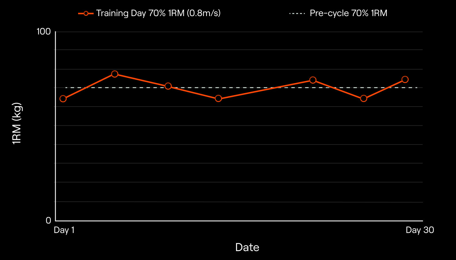
This can be very valuable when evaluating the effectiveness of your previous training decisions and when deciding on what to modify or do next. Therefore, we could easily abandon the idea of focusing only on our athletes’ percentages of 1RM and corresponding absolute loads and instead focus on their LVP. Shifting focus on our athletes’ or clients’ LVPs would mean that we could instruct them to find the absolute load that corresponds to a given movement velocity we want them to be lifting at. In Lorena’s example, if we wanted her to lift 70% of her 1RM, we would instruct her to find the load that she can lift at 0.8 m/s. After two-three single-set repetitions performed with maximal intent, she would know what is her 70% for the day and could then continue with her workout. We now see how we can use LVP to monitor training progress and prescribe training loads.

What’s next.

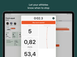
All right, we scratched the surface of using movement velocity to monitor and prescribe resistance training. We still need to cover quite a few things. For instance, we need to address how to use movement velocity to monitor the degree of fatigue incurred during resistance training, or how to use movement velocity cut-offs to terminate the sets. So, stay tuned!

References

1. Weakley, J., Mann, B., Banyard, H., McLaren, S., Scott, T., & Garcia-Ramos, A. (2021). Velocity-based training: From theory to application. Strength & Conditioning Journal, 43(2), 31-49.
2. Banyard, H. G., Nosaka, K., Vernon, A. D., & Haff, G. G. (2018). The reliability of individualized load–velocity profiles. International Journal of Sports Physiology and Performance, 13(6), 763-769.
3. Jukic, I., García-Ramos, A., Malecek, J., Omcirk, D., & Tufano, J. J. (2020). The use of lifting straps alters the entire load-velocity profile during the deadlift exercise. The Journal of Strength & Conditioning Research, 34(12), 3331-3337.
4. Marston, K. J., Forrest, M. R., Teo, S. Y., Mansfield, S. K., Peiffer, J. J., & Scott, B. R. (2022). Load-velocity relationships and predicted maximal strength: A systematic review of the validity and reliability of current methods. PLoS One, 17(10), e0267937.
5. Pestaña-Melero, F. L., Haff, G. G., Rojas, F. J., Pérez-Castilla, A., & García-Ramos, A. (2018). Reliability of the load–velocity relationship obtained through linear and polynomial regression models to predict the 1-repetition maximum load. Journal of Applied Biomechanics, 34(3), 184-190.
6. Banyard, H. G., Tufano, J. J., Weakley, J. J., Wu, S., Jukic, I., & Nosaka, K. (2020). Superior changes in jump, sprint, and change-of-direction performance but not maximal strength following 6 weeks of velocity-based training compared with 1-repetition-maximum percentage-based training. International Journal of Sports Physiology and Performance, 16(2), 232-242.